


The Multilayer Perceptron
Demystifying large language models, Part 1: How LLMs work


The Multilayer Perceptron
The generator/ decoder of LLMs is at its basis a ‘Multilayer Perceptron’ or MLP. Shy not away, perceptron is just a schmancy name for one of the most basic artificial neural networks, and we shall describe it all here.
The network's elemental node is the artificial neuron, inspired by the real biological neurons of the brain, and I'd like to begin with an introduction of this muse. It's not necessary to understand the biological to understand the artificial, but it doesn't hurt; I bring it as a bit of historical background. This is neuroscience's basic model of the nervous system, and I won't get into details that won't be directly relevant to the wider discussion.
The biological neuron is a somatic cell. Neurons communicate with each other. Each neuron has an ‘input end’ —branching extensions called dendrites— where it receives information and an ‘output end’ —a long extension called axon— through which it sends information to other neurons. This information is a simple binary signal, not unlike computer's ones and zeroes: either I'm on or I'm off.

Neurons are excitable, that is, they can get ‘activated,’ at which point they send a pulse down their axons, the action potential.1 Neurons get excited by other neurons, namely those that connect their axons to their dendrites. The interface between an axon and a dendrite is called synapse. Each incoming action potential shifts the neuron's electric potential a little bit. How much or how little varies depending on the strength of the connection, a strength referred to as weight. Once the accumulated shift of the neuron's electric potential goes past a threshold, it gets activated, sends its own pulse down its axon, then returns to a resting state.
Like the artificial neural network, and like the single neuron, our nervous system has an incoming end and and outgoing end. The afferent or sensory neurons receive information from the outside world: these are the photoreceptor cells in our eyes, the cells in our skin that are sensitive to pressure, to temperature, the chemical sensing cells in our nose, our tongue, our gut, the inner ear cells sensing the vibrations of the cochlear fluid and so on. Instead of being excited by other neurons, they get excited by whatever they are sensitive to: light, smell, touch. On the other end of our nervous system are efferent or motor neurons. Instead of sending pulses to other neurons, they send them to muscles that get contracted or relaxed and thereby move our limbs, our gut, our heart, our eyes, to glands that secrete hormones or sweat, and so on. And in between are the interneurons that meditate these two ends, and which compose most of our nervous system, including our brain.
The Multilayer Perceptron shares much with this model of the nervous system. It has neurons whose outgoing signals are provoked by incoming signals from other neurons. The connections have weights, which dictate how much influence an incoming signal has on the neuron. And the network as a whole has an incoming end and an outgoing end.
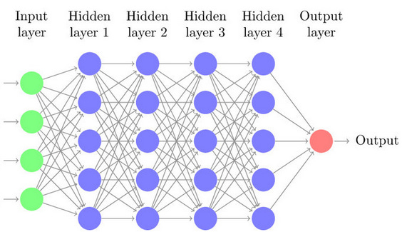
But there are major differences between the two. First, our nervous systems, and the brain in particular, has many recurrent connections. In other words, there are loops, such that following a path of neurons you might return to the beginning. There are indeed even neurons whose dendrites receive input from their own axons. In MLPs, however, information flows strictly in one direction. Their neurons are arranged in layers: there's the input layer that receives the network's input, the output layer that yields the output, and in between are interlayers that are ‘fully connected’: their neurons receive a signal from all the neurons of the previous layer and send a signal to all the neurons of the following layer.
Second, brains are spatial; the neurons composing them take room. Every neuron has limits, imposed by sheer consideration of space, on which and to how many other neurons it might be connected to. This is a distinction made not only vis-à-vis MLP, but simple neuroscientific models where, similarly to the fate of the spherical cow in physics, neurons lose their spatiality. Regardless, in artificial networks any neuron could be connected to any and as many other neurons as one fancies. In MLPs they are arranged in layers which dictate what neurons each neuron would be connected to, but the sizes of the layers —how many neurons make them up— is arbitrarily large.
In addition, the biological neuron's geometry affects its excitability by each of its dendritic synapses. This variability is captured by the modelled artificial weight, but one might speculate that there are dynamics which the static weight does not capture, and which might affect the emergent computations of the brain.
Third, related to the previous point, brains operate in time. It takes a while, albeit short, for signal to travel from one neuron to the next. MLPs (and artificial networks in general), on the other hand, have no temporality. They receive a single, discrete, input which they then process. It takes time for the MLP to run, but the duration has no effect on the process. Run the same network on a slow or a fast computer, you'd get the same result, just like two students who work on the same math problem at different speeds — assuming they make no mistakes. It's not a mere insignificant technicality. The nervous system continuously receives input from the environment, and it makes a difference how fast it processes it.2 Pain sensation takes several hundreds of milliseconds to reach from the toe to the brain; that's fast but not instantaneous, and things might happen in between which would influence the person's reaction to that pain. More obviously, our considerations take time, as well as energy, to the effect that sometimes the perfect comeback occurs to us first, too late, at the stairwell.
And fourth, artificial neurons do not use a binary but a continuous signal. Real neurons send forward either a 0 or a 1: ‘no action potential’ or ‘an action potential.’ Artificial neurons send a non-integer value whose range depends on their ‘activation function’; it might be any positive value, or a continuous value between -1 and 1, for example.3 Still, though it's continuous and not binary, the input-output relationship of their signals shares an important property with action potentials —namely non-linearity— discussed on the next post.

To make it more concrete, let's say we have an MLP which classifies b&w images of handwritten digits: the input is the image and the output is a digit from 0 to 9. We present it an image. In a manner of speaking, the image itself acts as a layer of the network, let's say it's the zeroth layer, with each of its pixels like a neuron. How black or white the pixel is corresponds to the outgoing signal of the neuron. A black pixel is like a neuron that outputs 0, a white pixel outputs 1, and shades of grey output a value in between, according to their brightness.
Each of the first layer's neurons receive the signal of each of the pixels (the zeroth layer's neurons), integrates them (sums them up in proportion to the weight it has with each pixel) and sends a signal to the next layer that is proportional to the sum.4 And so from one layer to the next until the final layer that has 10 neurons in it, each corresponding to one of the ten digits. The one that gets the strongest input is the one that has the final say, that outputs the ‘prediction’: the image is a 2, or a 7, or what have you.

Altogether, the MLP is like a voting system of sorts, a hybrid of referendums and a hierarchical representational democracy. At a referendum each voter can vote either ‘yes’ or ‘no.’ At a hierarchical representational democracy each voter elects a representative, each elected representative votes for a higher representative, who votes for a higher representative, and so on. The analogy is awkward, but hopefully adds comprehension somewhat:
At the bottom we have our constituency, of so and so voters. It's a referendum, and in addition to ‘yes’ and ‘no,’ each voter can vote ‘maybe’ of any interim degree. The voting is not equal: some votes have more power, represented by the weight. Though each voter participates in a single ballot, her vote —whether a yes, a no or a maybe— goes to all the referenda, as many referenda as there are neurons in the next layer, in each of which her weight would be different.
Next we have the second layer, another constituency whose voters cast their ballots based on the voting of the first constituency/ layer. Each voter corresponds to one of the previous referenda, and the more ‘yes’ she received, the more ‘yes’ she would cast on her own ballot. And so on and so forth until the last layer/ election where you have a competition and one individual wins the race, as it were.
It's a bizarre electoral system and you might wonder how this could work to classify written digits, to say nothing of its relation with LLMs.
For a first intuition, you might note that only the bottom constituency takes any independent decision, the rest merely follow the decisions already made for them. The final decision depends therefore on the bottom constituency's votes and on the voting power of each of the voters on each of the referenda throughout the system. In other words, the decision rests on the weights of the network and on the votes of the bottom constituency.
Second, imagine, again, that the bottom constituency is not the first layer of the MLP, but that zeroth layer, the input. Now the input represents the results of the round of ballots. Now the image is not a mere image, but a schema of our parliament, with each pixel representing a single chair, a single MP if you will. When we paint a pixel black, it's a chair that voted negatively, who blackballed the vote. If we paint a round black circle over the seats, we thus marked a group of dissenting voters. If we paint a straight vertical line, we marked a different, partially overlapping, group of voters. And so if we paint a black 7 or 8 or 9. In other words, each image defines what part of the constituency is voting positively and negatively, and if the system is rigged the right way, whatever part of the constituency votes ‘yes’ and ‘no’ would lead to the correct final decision.

The setup of the network layers' weight can be likened to gerrymandering. In gerrymandering electoral borders are redrawn to aggregate voters, based on demographic information, in such a way as to promote desired election results. Each interlayer artificial neuron is an aggregation of voters too: it has strong weights with some of the previous layer's neurons and weak weights with others. The weights are set in such a way that depending on the bottom constituency —the input— we get a desired outcome.
On the one hand, gerrymandering is easier: there's only one constituency, a single zeroth layer, and only one election that needs to be rigged, whereas the MLP's rigging needs to accommodate different zeroth layers —both the handwritten 7 and the handwritten 8, each of which has variations— to get correspondingly different electoral results — 7 or 8. On the other hand, gerrymandering is restricted at least by the requirement for electoral zones to be continuous, while in MLPs the connections can be arbitrarily set. In addition, the complicated one-ballot-several-votes and hierarchical elections makes possible a more complicated relationship between zeroth layer participation and final results.

It's not obvious how to rig the system to that effect —how to set the weights correctly— and it becomes more challenging as the classes (the categories being classified) grow more numerous and their distinction more complicated. It's one thing to yield a binary decision (as in machine learning models that predict anomalies in medical data —their presence/ absence— for example), another to choose from 10 possible results as in the case of the digit classifier, and yet another to pick from thousands of possibilities, as is the case with the LLM that decides on the correct ‘next word.’ As for the classes' complexity, I refer thereby to the relationship between the input's parts (e.g. pixel values) and the class. For example, the classification of b&w handwritten digits is relatively trivial, you could even describe in words that relationship. A single more or less vertical line with potentially a bit of a left leaning curve on top would be a 1; a single circle —a line that more or less loops on itself— would be a 0; two circles on top of each other would be an 8, and so on. You'd be hard pressed to do the same for a classifier of cat and dog images. Given the more variable morphology of dogs, the distinction between the two species is perhaps like the digits recognition where one digit is a cat and the rest are various dogs, from pugs and chihuahuas to Irish Wolfhounds and Great Danes. But let's say we just want to discriminate between cats and German Shepherds. The former have shorter snouts and relatively shorter legs. It's easy to put into words, but how do these correspond to pixel colour values?
If we had to set up the weights' values manually, we would not have gotten very far. To the rescue comes machine learning, the ability to ‘train’ the network on data: with a repeated trial-and-error process, the weights are marginally changed until we get weights that bring about the desired input-output relationship. More on that process in the over-next post.
It's not the most self explanatory term: the ‘action’ is an attributive noun, as in ‘action movie’; the ‘potential’ is ‘electric potential,’ for the signal is a drastic change in the cell's voltage.
In turn, this difference between the real nervous system and the MLP affect how the respective networks learn. Learning in the biological nervous system —the adapting change of weights between neurons— depends on the temporality of action potential events. As there's no temporality in the artificial neural networks, another technique must be employed, described on the over-next post.
The action potential is not a universal feature of biological nervous systems either. Some animals, such as the nematode C. elegans, have neurons that use a gradient signal as well.
Though the greater the sum the greater the outgoing signal, it is not exactly ‘proportional’; more on that in the next post.