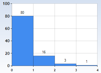
Neural networks model distribution, the way the bell curve might model human adult heights of a population: it charts the probability a member of the population picked at random would have a height within certain ranges. Picking many members it would illustrate the relative number of heights: you'd have about 5 persons of this height to every 4 persons of that height, for example.

Neural networks render a more sophisticated model still, of co-distributions, of distributions of one value given another value that has its own distribution. For example, the distribution of sex (about 1:1 male:female) and distribution of height are codependent, namely, adult females have a different height distribution than males, in most places shorter on average. We may include further properties still, such that fifteen year old males born in 16th century Netherlands have a different distribution of heights than sixty year old females born in 20th century China. Had we had the necessary statistics, we could have charted the appropriate bell curve for each combination of such demographic information.
An image classifier operates similarly, only it looks not on age, century of birth, sex, country of residence but on the red-blue-green value of pixel one, pixel two et cetera; it yields not a distribution of heights but of labels, say: 80% cat, 16% dog, 3% washing machine, 1% rake.

We could also pick at random a person of a selected height and look at another property of theirs. For example, we may look at the distribution of age among 20th century born, 165-166cm tall people, first among females, then among males; the latter distribution would be of younger people since there are far fewer adult males of that height than adult females. Or we could take just the height, 165-166cm and pick out one random person from all of recorded height history.
We could do likewise with the image model: we give it the label and it yields one random item from the distribution of images, i.e. codistribution of pixel values. If the previous model yielded a value for sex, age, century and so on given a height, this here yields a value for pixel one, pixel two and so forth given the label. This is how image generators work, very roughly. In practice it begins with noise, i.e. an image with random pixel values, and it iteratively changes these values towards an image that fits the label. e.g. cat. The colour values of each pixel are considered in the context of the other pixels as the ‘cat-ness’ of each pixel is not inherent, but contextual. To take a simpler example, whether a black pixel is part of a black line depends on other pixels, namely those that together would make a line if black, as well as their neighbours who would turn the line into another smudge if not white.
Before moving on to the second subunit of the LLM architecture, the word embedder, it would merit to say something about the relationship between the neural networks described so far and LLMs. After all, an LLM does not label data but generates text!
Though it might not look like it at first glance, the LLM operates similarly to any classifier, such as the image classifier. The difference is that the LLM returns a prediction in kind, and that it yields prediction iteratively while the image classifier yields a one off prediction. With the former I mean that the image classifier takes data of one kind and yield another, namely, it takes pixel values and yields a label. LLMs, on the other hand, take in text and output text. Second, the image classifier is done once it has yielded the label. An LLM makes a prediction —the next word— adds it to the end of the input text, and treats the new text as a new input for which it predicts yet another next word, and so on. Potentially it could do this forever. The kind of ‘LLM assistants’ that we love to hate and hate to love also predict when they should stop and pass the turn to the user — more on that in a future post about agency.
LLMs yield a particular text, but underneath every chosen ‘next word’ was a distribution from which the last layer of the network picked one word. If it has a vocabulary of 1000 words, given a text it would assign a probability for each of the 1000 items. During generation, a parameter called ‘temperature’ governs the policy by which the choice is made. On the lowest temperature the LLM behaves the most ‘conservative’ and always picks up the word with the highest probability as the next one, such that no matter how many times you prompted it with the same text, it will always complete it the same way. On the other end of the temperature spectrum you would get an LLM that completely ignores the distribution and randomly yields one of the 1000 vocabulary items with equal probability. And in between you get interim results: the next word is chosen randomly but with unequal probabilities that depend on the distribution.


